MODULES
Conjugate Natural Convection
Problem Definition: Case 1
In this problem three walls are of zero thickness and the right wall has some finite thickness 0.4 as shown in the Fig. 4.1. Horizontal walls are insulated and the right wall is at constant temperature 1 and left wall is at 0. For the solution, computational domain is divided into 9600 subdomains. Fluid domain is consist of 140×140 subdomains and the solid domain is consist of 60×140 subdomain. Clustering is done near the interface. This problem solved for the Gr = 105, (Ks/Kf ) = 2 and Pr = 0.71.
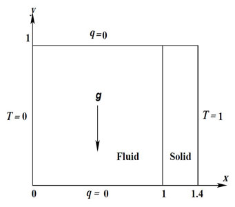
Figure 4.1: Sketch of the conjugate natural convection problem

The variation of temperature along the interface is shown in the Fig. 4.3 and compared with the Kaminski and Prakash [1] and found that temperature is not matching exactly. There is some disagreement between the result of Anupravaha and reference paper so the same problem is done by fluent software and result obtained from fluent is close to the Anupravaha result. So Difference between Anupravaha result and reference paper result may be due to the different schemes used for the solution or different mesh used.
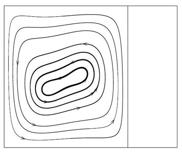
(a)
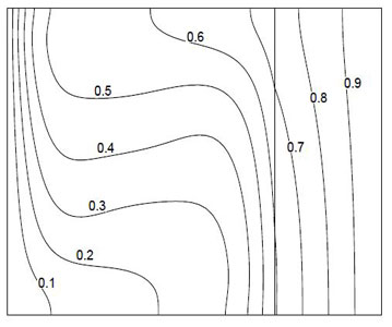
(b)
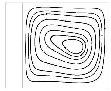
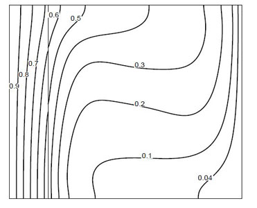
Figure 4.2: (a) Streamlines and (b) Isotherms
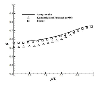
Figure 4.3: Temperature variation along the interface.
[1] Barletta A., Di Schio E.R., Comini G., and Agaro P.D. (2008) ‘Conjugate forced convection heat transfer in a plane channel:longitudinally periodic regime’, International Journal of Thermal Sciences, vol. 47, pp. 43–51.
The problem configuration is shown in the Fig. 4.4 In this problem, the cavity is heated at the left (solid wall) and cooled at the right side, and all other boundaries are insulated. All boundaries have no-slip velocity boundary condition. For the solution of this problem, the computational mesh consisted of 150 × 150 sub domains in the fluid part and 30 × 150 sub domains in the solid part of the domain is used. For the good solution clustering of meshes is done near the interface as shown in the Fig. 4.5. For the solution of the problem, the value of Pr is taken as 0.71 and Gr = 105 and characteristics length are considered as 1. The conductivity ratio is taken as 1 which is the ratio of thermal conductivity of solid to the fluid.
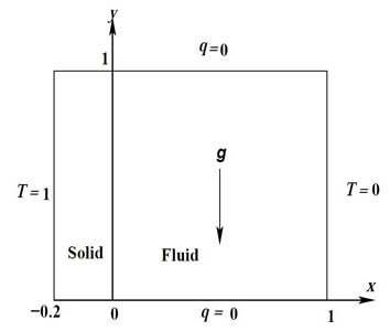
Figure 4.4: Sketch of the conjugate natural convection problem.
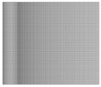
Figure 4.5: Meshing of computational domain
The streamlines and isotherm obtained from the solution are shown in the Fig. 4.6. The variation of temperature along the interface is compared with the result of Hribersek and Kuhn [2] in Fig. 4.7 and it is found that temperature variation along interface is matching with the reference result.
(a)
(b)
Figure 4.6: (a) Streamlines and (b) Isotherms
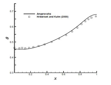
Figure 4.7: Temperature variation along the interface.
[1] Kaminski D.A. and Prakash C. (1986) ‘Conjugate natural convection in a square enclosure: effect of conduction in one of the vertical walls’, International Journal of Heat and Mass Transfer, vol. 29, pp. 1767–2010.
[2] Hribersek M. and Kuhn G. (2000) ‘Conjugate heat transfer by boundary-
domain integral method’, Engineering Analysis with Boundary Elements,
vol. 24, pp. 297–305.
