MODULES
Turbulent Flow Past A Triangular Cylinder
Problem Definition:
In the present study, an experimental case on flow past a built-in triangular cylinder (Sjunneson et al. [1]) has been validated. The flow domain, grid structure and boundary conditions have been chosen based on the data provided in Johansson et al. [2] and are shown in Fig. 2.1 and Fig. 2.2 respectively.
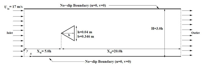
Figure 2.1: Flow Domain
The Reynolds number (Re) chosen for the flow is 45000, where the side-length of the cylinder (h) is chosen as the characteristic dimension. The upstream distance(Xu), downstream distance (Xd) and height of the domain are maintained as 0.2m, 0.8m and 0.8m respectively. Constant inlet velocity of 17m/s (with turbulent intensity (i)=5%) has been chosen as the inlet boundary condition. All turbulent variables are initialized with their inlet conditions with a slightly increased turbulent intensity (i). Time step chosen for the flow is 4×10⁻⁵. Standard κ− solver [3] with launder and spalding [4] wall function approach is used to resolve turbulent variables.
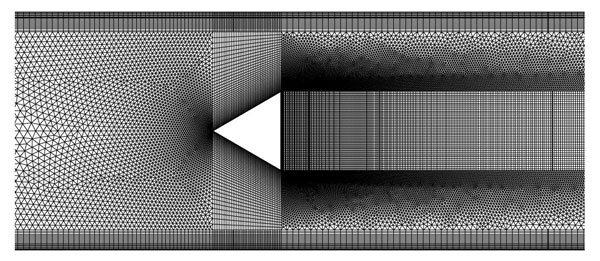
Figure 15.2: Computational Domain
The total no. of volume elements chosen are 80000 with a the distance of first cell-centre to wall to be 18 × 10−5m. The distance has been calculated from an online calculator based on y+ > 11.63.
Boundary Conditions:
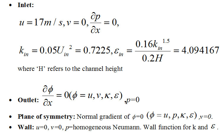

Figure 15.3: Phase-averaged instantaneous vorticity contour showing vortex strength  labels. Solid lines and dashed lines show counter-clockwise and clockwise rotating vortices respectively.
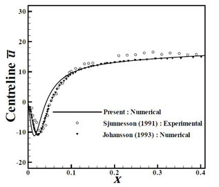
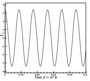
Time-averaged u-component of velocity is plotted along geometric centreline starting from the rear end of the cylinder. It can be well-comprehended from the Fig. 15.4 that present result has provided an accurate prediction of numerical re-sults of Johansson [1] in the far-wake region. However, it compares well with the experimental results. In the near wake region, ascribed to a poor prediction of cell-centre to wall distance (as it is done with the help of an online calculator which is based on the principle of flow over a flat plate), averaged u-velocity values in the near wall region is under-predicted. Table 15.2 shows the comparison of Strouhal number (St), which is a fairly good match. The time-period of shedding is found to be 0.0088 time units.
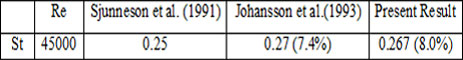
Table 15.1: Comparison of Present result with Johansson et al. [1] and Sjunnesson et al. [2] for Strouhal Number
(a)
(b)
Figure 15.4: (a) Time-averaged centreline u-velocity vs x, (b) Cl vs Non-dimensional time (t*) showing the periodic fluctuation of lift-coefficient
[1] Johansson S.H., Davidson L., and Olsson E. (1993) ‘Numerical simulation of vortex shedding past triangular cylinders at high reynolds number (Re) using a κ − turbulence model’, Int. J. Num. Meth. fluids, vol. 16, pp. 859–878.
[2] Sjunnesson A., Nelson C., and Max E. (1991) ‘LDA measurements of velocities and turbulence in a bluff body stabilized flame’, Laser Anemometry, vol. 3, pp. 83–90.
[3] Naik A.K. (2015) ‘Implementation of isotropic eddy viscosity turbulent models over hybrid unstructured grid’, M.Tech Thesis, Department of Mechanical Engineering, Indian Institute of Technology Guwahati.
[4] Launder B. and Spalding D. (1974) ‘The numerical computation of turbulent
flows’, Comput Method Appl M, vol. 3(2), p. 269289
