MODULES
Conjugate Forced Convection In A Channel: Half Domain And Constant Temperature Boundary
Problem Definition:
Problem configuration is shown in the Fig. 1.1, velocity inlet is parabolic and channel walls are at constant temperature 1 and at the walls no slip boundary condition is applied. The problem is symmetric so we can solve the half channel for the solution. For the solution, half channel is taken and computational domain is divided into small subdomains. The computational mesh consist of 100×20 subdomains in the fluid region and 100×10 subdomains in the solid region with clustering near the interface as shown in the Fig. 1.2. The inlet velocity is u = 6(1.5 − y)(y − 0.5). For the solution of the problem, the parameter taken as Pe = 50 and conductivity ratio (K) is 1. Mean velocity 1 and channel height is used for the calculation of Pe number.
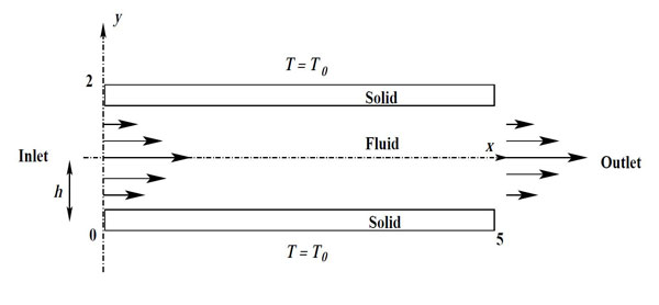
Figure 1.1: Sketch of the conjugate forced convection problem
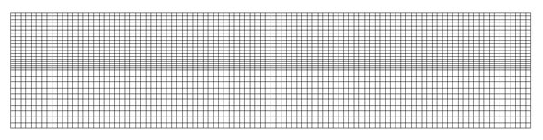
Figure 1.2: Meshing of computational domain.

In Fig. 1.4 the comparison of interface temperature with the Hribersek and Kuhn [1] and it is found that it is matching. There is a very small gap in tem- perature this is due to the different schemes used, they have used boundary de- composition method for the solution.
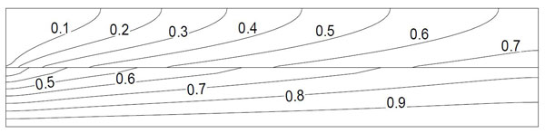
Figure 1.3: Isotherms
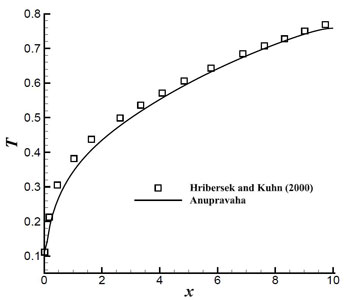 Figure 1.4: Temperature variation along the interface
[1] Hribersek M. and Kuhn G. (2000) ‘Conjugate heat transfer by boundary-domain integral method’, Engineering Analysis with Boundary Elements,vol. 24, pp. 297–305.
