MODULES
Two-Dimensional Bubble Rise
Problem Definition:
The problem defines a two-dimensional bubble with an initial radius of 0.25, centered at (x, y) = 0.5, 0.5 in a quiescent medium as shown in Fig. 2.1. The size of the computational domain is 1 × 2 and is discretized into 5000 hexahedral cells with a uniform grid spacing of 1/50. Hysing et al. [2] performed this numerical experiment with two different sets of properties, one with a large variation in density and viscosity ratio, while the other one is for a lesser property variation. Here we present the results for the case with higher density ratio, as it is more significant as compared to the one with lesser property variations. Physical parameters for this case are ρ1 = 1000, ρ2 = 1, μ1 = 10, μ2 = 0.1, g = 0.98 and σ = 1.96.
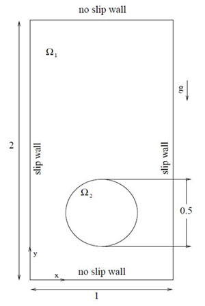
Figure 2.1: Computational domain for 2D bubble rise problem with initial set up and boundary conditions. 1 and 2 are the regions of heavier and lighter fluid respectively.

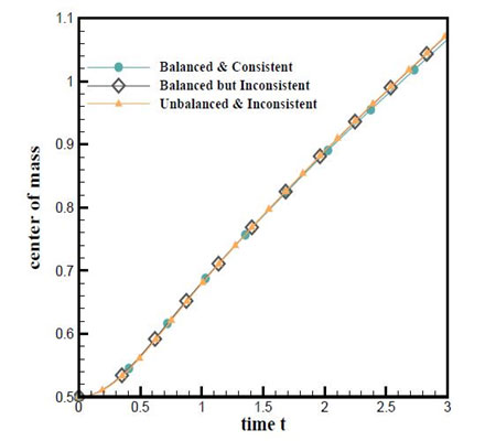
(a)
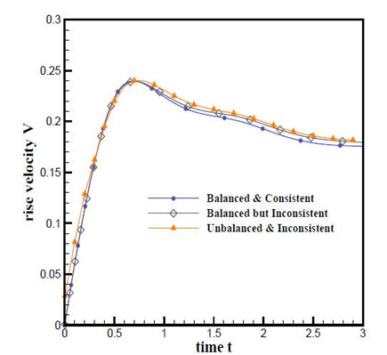
(b)
Figure 11.2: Temporal evolution of (a) center of mass and (b) rising velocity for 2D bubble rise problem.
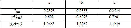
Figure 1.4: Comparison of dam front
[1] Klostermann J., Schaake K., and Schwarze R. (2012) ‘Numerical simulation of a single rising bubble by vof with surface compression’, Int. J. Numer. Meth. Fluids, vol. 71, pp. 960–982.
[2] Hysing S., Turek S., Kuzmin D., Parolini N., Burman E., Ganesan S., and
Tobiska L. (2008) ‘Quantitative benchmark computations of two-dimensional
bubble dynamics.’, Int. J. Numer. Meth. Fluids, vol. 60, p. 2591288.
